Case of an incoherent illumination

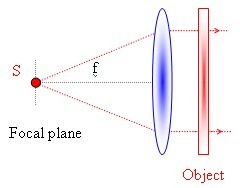
In the case of a (spatially) coherent illumination (see figure V-3), the complex amplitudes at all object points follow the same evolution with time.

Experimentally, this is realized by placing a light source of small dimension at the front focal plane of a lens.

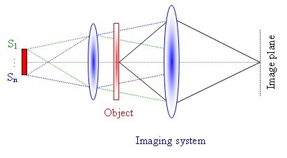
The illumination is said to be spatially incoherent is the source is (spatially) wide enough (see figure V-4).

The complex amplitudes of all points forming the source vary on a random fashion, and independently from one another. There is no fixed phase relationship between a wave train emitted by S1 and another one emitted by Sn and the temporal average over the interference term is equal to zero.

In the case of an incoherent illumination, we have to sum the intensities, and not the fields.

The image is therefore written as a linear transformation of the intensity [] :

The image intensity is a convolution between the ideal intensity (obtained with geometric optics) and a point spread function proportional to the square modulus of the point spread function obtained with coherent illumination.

We define the normalized spectra of Ig and Ii :

The spectra are normalized with respect to the integral value at zero frequency, which represents the continuous component or background of the image.

In a similar fashion, we define the normalized transfer function of the system:

By applying the convolution theorem to Eq. V-2, we obtain:

is called «optical transfer function» («OTF») or «modulation transfer function» («MTF»).

Using the autocorrelation theorem:

By applying the change of variables u''=u'-u/2 and v''=v'-v/2 , we obtain a symmetrical expression:

For a coherent system, we have , and therefore we obtain:

where we replaced u'' with u' and P² by P in the denominator (since P=1 or 0). The relation (V-3) serves as a fundamental link between coherent and incoherent systems.

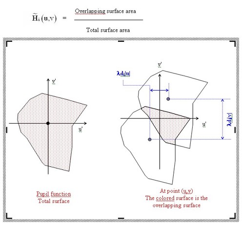
In the expression of appears the area of the common surface between two identical pupil functions:

• one centered at the point of coordinates : ,

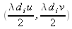• the other centered at the diametrically opposed point, of coordinates : .

The denominator normalizes this area with the total pupil area (see figure V-5).

For more details pertaining to this subject, the reader can refer to [ ] and references therein.