Fraunhofer diffraction of a sinusoidal amplitude grating

Until now, the aperture transmittance t(x,y) was a binary function (taking 0 values outside the aperture and 1 values inside). However, we can introduce absorbing spatial distributions (for example using a photographic film) and thereby obtain all transmittance values ranging between 0 and 1.

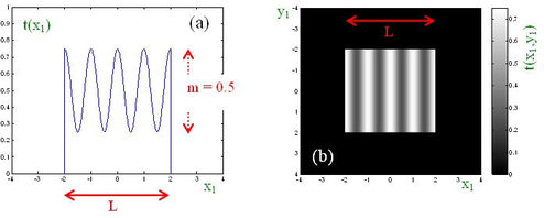
We consider a sinusoidal amplitude grating limited by a square aperture of side length L :

where f0 is the spatial frequency of the grating and m represents the peak-to-peak variation of the amplitude. m is called the amplitude modulation depth (see figure EC1(a)).

Figure CS1(b) shows the grating image. Of course, the grating step has been voluntarily increased in this figure to visualize the sinusoidal transmittance.

If the screen is illuminated under a normal incidence with a monochromatic plane wave of unit amplitude, the field distribution at the aperture is simply equal to t(x1,y1).

The Fraunhofer diffraction figure can be determined through the calculation of FT (t) :

We define:

Using the distributivity property of the convolution product, we can write:

Considering that translating a function f(x,y) of a quantity a is equivalent to taking its convolution with the translated Dirac delta function (δ(x-a)) :

we obtain:

We can deduce the field distribution in amplitude:

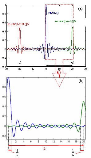
In figure CS2(a), we represented the 3 sinc functions centered at -f0, 0 and +f0 in the case where m=1.

An enlargement of this figure is shown on figure EC2(b) where we can see the central peak widths of the two sinc functions centered at 0 and +f0.

If , the product of those two functions can be neglected, because when one function reaches its maximum the other takes values close to zero. We can therefore neglect the overlap between the 3 sinc functions. When calculating the intensity, the cross-products between these functions are negligible compared to the square of each of these functions.

Finally, the intensity in the observation plane becomes:

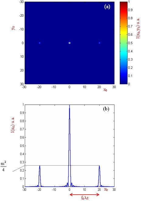
An image of the diffraction figure obtained using this latter equation is shown on figure CS3(a).

A part of the light is deflected in two lateral lobes. The central part is called zero-order component and the two lateral lobes are called 1st order components. Figure CS3(b) represents the evolution of the normalized intensity for y0 =0 and m=1. We can note that the distance between the first order diffraction lobes and the central lobe is f0λz. In addition, in the best case (when m=1), the intensity in the diffracted lobes cannot exceeds 0.25 for a grating sinusoidal in amplitude.