Methods for reconstructing the object wave front
Introduction
Two methods are presented in this chapter :
-
The reconstruction of the complex object field by the Fresnel transform ;
-
And the convolution reconstruction method.
Both are based on the Fresnel-Kirchhoff diffraction integral.
Reconstruction using a discrete Fresnel transform
Let's consider that instead of a classic diffracting aperture that we have a discrete transmittance; this represents a hologram recorded beforehand on a pixel matrix. We have already seen that the object wave is reconstructed by diffracting the reference beam onto the holographic plate. In order to obtain phase and amplitude information from the initial field, the diffraction of the incident reference wave must be simulated on the transmittance matrix.
The Fresnel diffraction integral is discretised by replacing the double integral with a double summation and the recording plane coordinates are sampled with a pitch which corresponds to that of the pixel matrix, that is to say
 , where
 and
and
 vary from 0 to
 and from 0 to
 .
.
Also, since the processor cannot calculate an infinite number of points in the reconstructed field, the discreet nature of the image plane must also be taken into account. In particular, it is necessary to consider the nature of the Fresnel integral: it is a two-dimensional Fourier transform. The classic rules for time and frequency sampling which are applied to the digital processing of the classic signal are also essential in this case. For the recording of a digital hologram at a reconstruction distance
 , the discret eFresnel transform is written :
At this point, it must be noted that in this calculation it is not obligatory to take the reference beam into account if it is plane and uniform
 , contrary to the case of physical reconstruction using a laser which requires illumination with a reference beam. In the case of a spherical wave
 , it would be necessary to take the curvature of the wave front into account and to multiply
 by an appropriate complex term.
The discretisation of the reconstructed plane
According to the expression for the discrete Fresnel transform, the apparent sampling periods of the exponential function, which gives the Fourier character of the integral, are shown by :
If the reconstructed field is calculated using the same number of points
 that is pixels in the detector, the sampling pitch in the image plane is equal to :
Consequently, the sampling in the image plane is simply :
where
 and
and
 vary from
 and from
 .
.
Zero-padding (extending the pixel matrix with zeros) will be discussed later on. The discrete version of the Fresnel integral is ultimately written :
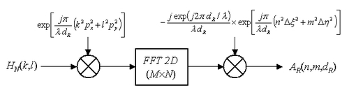
This relationship expresses the reconstructed field at the pixel coordinates
 in the image plane. With only one phase factor, the reconstructed field is proportionate to a discrete two-dimensional Fourier transform (FFT = Fast Fourier Transform) of the product of the digital hologram multiplied by a discrete quadratic phase term.
The algorithm for reconstruction using the discrete Fresnel transform is shown in figure 15.
![[zoom...]](javascript:window.open(%22../res/Fig_15_1.jpg%22,%22_blank%22,%22width=%22+Math.min(800,screen.availWidth)+%22,height=%22+Math.min(600,screen.availWidth)+%22,left=%22+(screen.availWidth-800)/2+%22,top=%22+(screen.availHeight-600)/2+%22,scrollbars=yes,resizable=yes%22)?void(0):void(0))
If one were to choose
 , then the +1-order would be in focus in the reconstructed field. If, on the other hand, one were to choose
 , it would be the -1-order that was in focus.
Constraints on the reconstruction distance
The reader should note that the application of this algorithm requires a discrete version of the quadratic phase term of the Fresnel transform to be programmed. The sampling of this complex oscillating function is necessary in order to respect the Shannon conditions.
In order to do this, one only needs to consider the spacial frequency content of the function in terms of spatial frequencies []. Let's consider the phase of the quadratic term :
The spatial frequencies are given by :
Giving
The quadratic term is a signal with an unstationary character since its frequencies
 vary according to the evolution variables
 . In theory, the energy of the signal is infinite.
However, the signal must be considered within the confines of a limited space – that of the sensor's pixel space. Delimiting its evolution horizon imposes a limit on its energy and on its frequential content. The size of x and y is restricted by
 and
and
 which correspond to the recording scale (
 pixels at a pitch of
 , sensor
 ), this is to say
 and
and
 .
.
Thus, the maximum spatial frequencies of the signal are given by :
Within the sensor, the bilateral spatial bandwidth of the quadratic term is therefore :
Thus, the bandwidth reduces when the distance increases. The Shannon theory imposes the following :
Since the pixel pitch is imposed by the technology being used, the minimum distance
 which represents the Shanon criteria is given by :
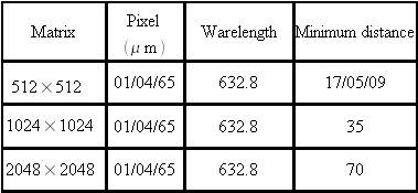
Table 2 sums up the minimum distances according to the acquisition parameters.
![[zoom...]](javascript:window.open(%22../res/tablo_02_1.png%22,%22_blank%22,%22width=%22+Math.min(800,screen.availWidth)+%22,height=%22+Math.min(600,screen.availWidth)+%22,left=%22+(screen.availWidth-800)/2+%22,top=%22+(screen.availHeight-600)/2+%22,scrollbars=yes,resizable=yes%22)?void(0):void(0))
This result imposes a minimum distance for reconstruction using the Fresnel transform.
Expression of the digital +1-order
The analytical calculation of the diffracted field in the +1-order must take into account the active pixel surface, the comparative lack of focalization in digital holography and the possible surface aberration of the reference beam. This calculation will not be analysed in this course. Instead, we have settled for outlining the principal result in the case of the pixel being infinitely localised
 and for
 where we have
 .
.
From the equation of the discreet Fresnel transform, we get that the digitally diffracted field in the +1-order is shown by :
With
And
 is the two-dimensional Dirac distribution. The +1-order is therefore located at the coordinates
 in the reconstructed plane. These coordinates depend on the spatial frequency of the reference wave and the reconstruction distance.
As we saw in paragraph A.2.c, the reconstructed object is also convoluted by an enlargement function
 which is linked to the size of the sensor. This function is the filter function of the two-dimensional discrete Fourier transform. Its mathematical form seems very different from that of the function
 , however, its profile is similar to a two-dimensional sinc function.
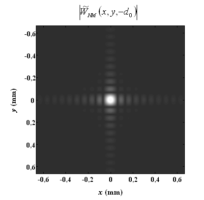
This function imposes the pre-defined resolution on Fresnel digital holography. The interpretation of this function is quite simple :
 is a digital diffraction puttern of a rectangular aperture of dimensions
 with uniform transmittance. The resolution function is graphically represented in modulus in figure 16 for the following digital values :
 ,
,
 ,
,
 and
and
 .
.
![[zoom...]](javascript:window.open(%22../res/Fig_16_1.jpg%22,%22_blank%22,%22width=%22+Math.min(800,screen.availWidth)+%22,height=%22+Math.min(600,screen.availWidth)+%22,left=%22+(screen.availWidth-800)/2+%22,top=%22+(screen.availHeight-600)/2+%22,scrollbars=yes,resizable=yes%22)?void(0):void(0))
According to the Raleigh criteria, this function has widths equal to :
These quantities set the resolution in the image plane. The spatial resolution is therefore proportional to the recording distance and inversely proportional to the width of the sensor.
A digital application with the values given above produces
 . In comparison with digital applications with a silver plate of
 , the spatial resolution is 21 to 25 times smoller.
Getting rid of the interference orders
The algorithm shown in figure 15 can be directly applied to the recorded hologram. In this case, the reconstructed field will systematically contain the three diffraction orders. In 1997 [], Yamaguchi proposed applying the technique of fringe demodulation by phase shift to digital holography. The idea is that since the hologram is an interferometric composition of two waves, it is possible to extract the desired order by applying a phase shift to the reference wave.
Note that
 is the phase shift applied to the reference wave which is now written :
Let's choose 4 phase shift values :
Then, since H can also be written
We can extract from each of the four recorded holograms, the phase of the diffracted object field
 and its amplitude
 and we can also calculate the +1-order which corresponds with the term
 . In fact at each point where the hologram is recorded :
And
Then, applying the algorithm we have seen in figure 15 to the -1-order is all that is needed to form the image of the initial object on its own. This method is efficient as far as getting rid of the +1-order is concerned but it is over-the-top in recording terms since four holograms are re1quired to reform the object.
Zero-padding
It should be remarked that the sampling pitch of the image space depends on the number of points used in the reconstruction, on the wavelength, on the pixel pitch and on the reconstruction distance. There is therefore no invariance in the sampling pitch at the moment of reconstruction by the direct Fresnel transform.
As has been mentioned in one of the previous paragraphs, the diffracted field is estimated over a finite number of points. The calculation of the discreet Fresnel transform of the hologram can be carried out over points
 as
as
 .
.
-
If
 then the raw interferogram is used in the digital calculation of the Fresnel transform.
 -
If
 one finds oneself in the situation of zero-padding (which basically means adding
 zeros to the pixel matrix).
Fundamentally, these additional zeros do not add any rational information but they do modify the sampling pitch of the diffracted field.
Indeed, the pitch would now be given as :
The sampling in the image plane is henceforth :
Where
 and
and
 vary from
 and from
 .
.
We therefore know that
 and
and
 . There is a reduction in the sampling pitch and thus an increase in the “definition” of the image plane.
In concrete terms, this means that we see a greater texture in the image : the zero-padding of the hologram has the consequence of making the speckle grain structure of the image appear more precise.
However, zero-padding does not change the intrinsic resolution which is imposed by the number of pixels in the image sensor and the size of these pixels.
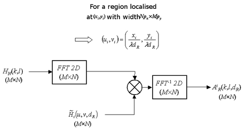
Reconstruction by convolution
Let's look again at the Fresnel-Kirchhofff diffraction integral expressed in Cartesian coordinates[] :
This integral is also a convolution equation :
With
 , the impulse response of the free space propagation, expressed by :
In the framework of the Fresnel approximations, the impulse response becomes :
And the diffracted field is expressed by the Fresnel transform which we have already seen at the beginning of this course :
The impulsional response has a transfer function
 so that :
Applied to the reconstruction of the object field at the distance
 , from the hologram
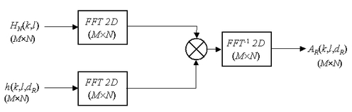
 , the discreet version of the convolution equation is simply :
There are several ways to look at the practical use of this relationship. The simplest is to use the properties of the Fourier transform: the convolution of two functions can be processed by the inverse Fourier transform of the product of the Fourier transforms of each of the functions.
This property is used in digital holography, given that calculation by discrete Fourier transforms is less time consuming in terms of calculation than the convolution method (double summation as opposed to optimised algorithms).
Thus the reconstructed field at the distance
 is calculated by application of the following equation :
The algorithm for reconstruction by discrete convolution is given in figure 17.
![[zoom...]](javascript:window.open(%22../res/Fig_17_1.jpg%22,%22_blank%22,%22width=%22+Math.min(800,screen.availWidth)+%22,height=%22+Math.min(600,screen.availWidth)+%22,left=%22+(screen.availWidth-800)/2+%22,top=%22+(screen.availHeight-600)/2+%22,scrollbars=yes,resizable=yes%22)?void(0):void(0))
It is possible to apply this algorithm to just the +1-order, extracted from the hologram by the phase shift technique.
The reader should note that the reconstruction conditions which were outlined in the previous paragraph and which concern the minimum recording distance
 are also valid in this case. If the exact impulse response [] is used we get :
Let's consider the algorithm from figure 17: two Fourier transforms are used; a direct transform and then a reciprocal one. Because of this, the observation horizon of the reconstructed field is identical to that of the recorded hologram. This means that the sampling pitch in the image plane is identical to the pixel pitch, that is to say
 and
and
 contrary to the case of direct calculation where the pitch depends on the reconstruction distance.
This method is thus recommended when the sampling pitch needs to stay constant in the different reconstructed planes.
Spectral scanning by the filter bank method
With the FFT digital convolution method, the maximum observation horizon is imposed by the size of the sensor matrix. If the object is larger than the pixel matrix, it is necessary to carry out a spectral scan in order to reconstruct the object by assembling adjacent pieces. In terms of spatial bandwidth, this means that the bandwidth of the impulse response is not sufficient to cover the spatial bandwidth occupied by the object. In this case, in order to put into place a reconstruction by convolution it is necessary to programme the filter bank so that its role is to carry out the spectral scanning which is necessary for the reconstruction of the whole object.
The number of required scans depends on the bandwidth of the filter. The relationship between metric space and spatial frequency shows that a holographic spatial frequency equal to
 matches a point in the reconstructed object equal to
 . The bandwidth of the impulse response allows an area, equal to
 in width and
 in height, to be reconstructed in a single operation. If the object is of a span
 greater than
 the number of required horizontal scans is given by the spectral bandwidth ratio, which is to say :
It is simply equal to the sensor size/object size ratio. A similar relationship exists between the vertical scanning and
 .
.
If the spectrum of the diffracted object wave is located at the frequential coordinates
 , the spatial frequencies of the filter bank are given in the two directions by :
With
The algorithm for spectral scanning is given in figure 18.
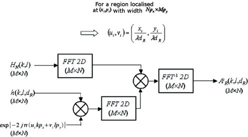
![[zoom...]](javascript:window.open(%22../res/Fig_18_1.jpg%22,%22_blank%22,%22width=%22+Math.min(800,screen.availWidth)+%22,height=%22+Math.min(600,screen.availWidth)+%22,left=%22+(screen.availWidth-800)/2+%22,top=%22+(screen.availHeight-600)/2+%22,scrollbars=yes,resizable=yes%22)?void(0):void(0))
The form of the algorithm is the result of the properties of the Fourier transform regarding the spectral shift induced by the modulations in the direct space.
In order to reconstruct a region of the object whose central coordinated are
 are and whose size is equal to that of the sensor
 , the central spatial frequency associated with that area is calculated ; that is to say
 . The spectral filter associated with this area must therefore be focused on the coordinates in the spectrum of the hologram. The spectral alignment is thus carried out by modulation of the impulse response of the free space using numerical calculation :
Thus, the transfer function associated with the impulse response modulated by the spatial frequency in the spectral zone is :
With this transfer function, multiplied by the hologram spectrum, only the spectral zone of interest is kept. Thus, through spectral scanning by the filter bank method, the object can be reconstructed in its totality.
The larger the object in comparison to the size of the sensor, the more it is necessary to carry out the calculation using filters and the longer the reconstruction takes. In addition, the final image is obtained by the juxtaposition of adjacent reconstructed pieces: the size of the object image is now thus
 pixels. If the number of scans imposes a final image size greater than
 pixels, the memory space being used will be considerable which will limit the possibilities for digital treatment of the obtained results.
Other strategies
Other reconstruction strategies exist which are based on the convolution equation. From the expression of the impulse responses and the associated transfer functions [], two other reconstruction methods can be distinguished :
-
A filter bank derived from the exact form of
 with
with
-
A filter bank derived from the expression of
 in the Fresnel approximations with
Taking into account the fact that spectral bands are finite in digital holography, these two expressions need to be adapted, firstly by limiting their spectral range and also by focusing their transfer function on
 .
.
Thus they become respectively :
And
Figure 19 represents the reconstruction algorithm with the transfer functions.
![[zoom...]](javascript:window.open(%22../res/Fig_19_1.jpg%22,%22_blank%22,%22width=%22+Math.min(800,screen.availWidth)+%22,height=%22+Math.min(600,screen.availWidth)+%22,left=%22+(screen.availWidth-800)/2+%22,top=%22+(screen.availHeight-600)/2+%22,scrollbars=yes,resizable=yes%22)?void(0):void(0))
The method resembles that which was outlined in the previous paragraph and therefore the number of scans and the final image sizes are identical.
Methods of digital reconstruction by convolution are currently used in digital holographic microscopy : imaging using phase polarization or phase contrast [] and also in 3D microscopy [,]. Indeed, reconstruction in different adjustment planes is only appropriate if the sampling pitch of the image remains constant.