Sampling and quantization
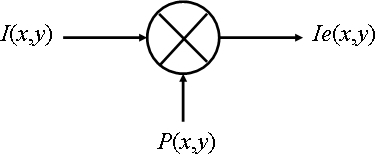
Before being processed by a computer, the analog images must be sampled and quantified. Here, we consider the ideal case of image sampling. The ideal sampler model is a simple product of the initial image with a bidimensional comb function. This calculation yields a sampled image Ie(x,y) whose values correspond to the luminance registered on a regular grid of parameters
 .
.
![[zoom...]](javascript:window.open(%22../res/Figure-II-4-1_1.jpg%22,%22_blank%22,%22width=%22+Math.min(800,screen.availWidth)+%22,height=%22+Math.min(600,screen.availWidth)+%22,left=%22+(screen.availWidth-800)/2+%22,top=%22+(screen.availHeight-600)/2+%22,scrollbars=yes,resizable=yes%22)?void(0):void(0))
Expression of the sampled image:
The weights I(mDx, nDy) associated with the delta functions are the pixels of the image. Shannon theoem extended to 2 dimensions is written on the same way as in the monodimensional case, except that here we find an additional degree of freedom in the geometry of the 2D sampling pattern. However, in this lesson, we will not detail this point and we will limit ourself to a regular sampling pattern.
An analog image I(x,y) imited to the spatial frequencies Xmax and Ymax can be reconstructed using the sampled data
 if the sampling periods verify:
In order to understand the frequency representation of the sampled image, we first need to compute its Fourier Transform. We thus note:
Replacing Ie(x,y) by its expression yields a double integral of a double discrete sum. By linearity, we can permute the summation and integral signs to obtain:
In the integral term, we recognize the Fourier transform of a delta function translated by a quantity
 . By choosing unit values for
 ,we finally obtain:
This is the simplified form of the bidimensional Fourier transform applied to discrete images. To understand the relation between the spectra of digital and analog images, we can notice that the image Ie(x,y) is the product between the analog image and the bidimensional comb function, and therefore its Fourier transform is the convolution product of the Fourier transforms of the image F(u,v) and of the comb:
Therefore:
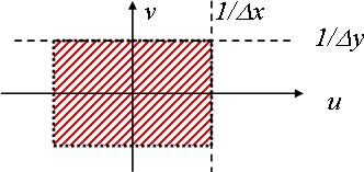
Consequently, Fe(u,v) results from the periodization of the pattern formed by F(u,v) along the axes u and v. Fe(u,v) is a doubly periodic function of periods
 . It can be represented without any information loss by restricting the (spatial) frequency space to a rectangular cell of dimensions
 centered for example at zero frequency (0,0). The figure below shows the domain of definition of Fe(u,v) restricted to this one period.
![[zoom...]](javascript:window.open(%22../res/Figure-II-4-2_1.jpg%22,%22_blank%22,%22width=%22+Math.min(800,screen.availWidth)+%22,height=%22+Math.min(600,screen.availWidth)+%22,left=%22+(screen.availWidth-800)/2+%22,top=%22+(screen.availHeight-600)/2+%22,scrollbars=yes,resizable=yes%22)?void(0):void(0))
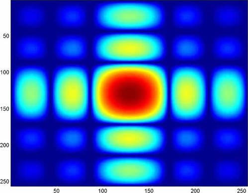
We consider a bidimensional discrete rectangular function R(m,n) such that:
By using the discrete FT expression, we obtain:
After separating the exponential term, we find that Fe(u,v) if the product of two partial sums of well-know series. By calculating these terms, we finally obtain:
![[zoom...]](javascript:window.open(%22../res/Figure-II-4-3_1.jpg%22,%22_blank%22,%22width=%22+Math.min(800,screen.availWidth)+%22,height=%22+Math.min(600,screen.availWidth)+%22,left=%22+(screen.availWidth-800)/2+%22,top=%22+(screen.availHeight-600)/2+%22,scrollbars=yes,resizable=yes%22)?void(0):void(0))
When an image is sampled without satisfying Shannon criteria, the various replica of the initial image spectrum overlap, causing the so-called aliasing phenomenon (or “moireing”, in the case of images). To evidence this phenomenon, a technique consists in under-sampling an image constituted by a line grating, as shown in the following example:
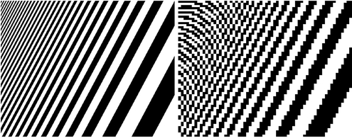
![[zoom...]](javascript:window.open(%22../res/Figure-II-4-4_1.jpg%22,%22_blank%22,%22width=%22+Math.min(800,screen.availWidth)+%22,height=%22+Math.min(600,screen.availWidth)+%22,left=%22+(screen.availWidth-800)/2+%22,top=%22+(screen.availHeight-600)/2+%22,scrollbars=yes,resizable=yes%22)?void(0):void(0))
In relation to image representation in a computer, image Ie(x,y) can be seen a series of delta functions: each delta function is located at the center of a pixel and has an amplitude corresponding to the pixel intensity; the rest of the pixel has an intensity equal to zero. The pixel representation corresponds to filtering the image Ie(x,y) with a rectangular filter whose impulse response is centered at the origin and has a size equal to the pixel size.
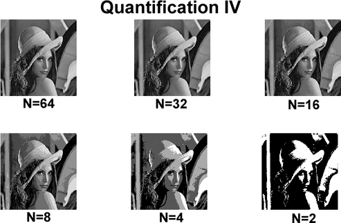
The sampling process is complemented by a quantization process, which associates a discrete value to the pixel intensity. Most of the time, the cardinal number of this ensemble of discrete values is related to the binary representation used for storage. The quantization process consists in dividing the luminance dynamic range D in a finite number of intervals. The dynamic range is determined by the physical support of the information before digitalization. The problem is then to appropriately choose the number of quantization levels. A bad choice leads to artificial outlines in the image corresponding to steps between quantization levels. The quantization interval must be chosen smaller than a quantity called luminance liminar step Cw, which represents the minimum luminance variation perceptible by a typical observer. The minimum number of levels Nq can then be expressed as a function of the dynamical range D (expressed in optical density units) and the step Cw:
Using the values: D = 2 for a photograph and Cw = 0.01 for a good observer, we obtain:
This leads to using N = 512 levels, i.e. 9 bits of quantization to code the various pixels. The same calculation performed for a medium observer (Cw = 0.02) leads to N = 256 levels, i.e. 8 quantization bits, or a byte. This is the most frequently used value for multimedia applications.
![[zoom...]](javascript:window.open(%22../res/Figure-II-4-5_1.jpg%22,%22_blank%22,%22width=%22+Math.min(800,screen.availWidth)+%22,height=%22+Math.min(600,screen.availWidth)+%22,left=%22+(screen.availWidth-800)/2+%22,top=%22+(screen.availHeight-600)/2+%22,scrollbars=yes,resizable=yes%22)?void(0):void(0))