Signal to noise ratio and optimization

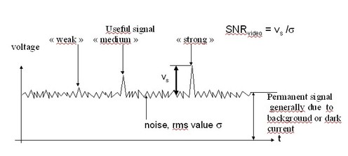
In quite many applications, noise adds to the useful signal, while in others, noise is proportional to signal. Whatever the case, the larger the noise fluctuations, the more difficult it is to detect or measure the useful signal. Figure 14, which shows a typical detector output with respect to time, is intended to illustrate the fact that the performance of an electro-optical sensor does not depend on its signal alone but on its signal to noise ratio.

Since the sensor output is noisy, it fluctuates above and below its average value by an instantaneous amount, for example ib (t) if one is concerned with the output current. The corresponding current or voltage variances, σ2i or σ2v, inside the electronic bandpass of the sensor generate the following electrical noise power Pn across the load resistor RL:

If is is the instantaneous pertinent output from the detector, the corresponding electric power of the signal is :

By definition, the power signal to noise ratio of the sensor at that corresponding instant is the ratio between the electrical pertinent signal power and that of the noise, both being evaluated inside the sensor bandpass:

Spatial (geometric) and spectral filtering are aimed at minimizing shot noise, due for example to stray light, and at maximizing lens transmittance for the pertinent signal.

• In infrared sensors, one will limit field of view of the (cryogenically cooled) detector to the exit pupil of the associated lens, in order to reduce its sensitivity to stray light radiated by the mechanical parts, main source of noise.

• Whenever possible, one will eliminate stray light from intense sources of light outside the field of view, by means of diaphragms, baffles, or protective screens.

• Early infrared missile guidance sensors were using finely etched rotating graticules aimed at reducing signals from extended sources such as clouds.

• In image forming sensors, the elemental field of view must be matched to the size of the finest details to be detected on the object.

The spectral bandwidth of the sensor must be optimized with respect to the signatures of useful and parasitic radiations. Spectral filtering is most efficient in active sensors (particularly laser sensors) since the signal to detect is then monochromatic, while stray light is usually spectrally wide. Under these conditions, interference filtering is recommended : centered upon the laser wavelength it will isolate a narrow bandpass : relative width (Δλ/λ) less than or of the order of 1% is rather commonplace.

If the sensor operates in the long wave IR band (8 to 12 µm band), one may also use filters, but then they should be cooled down at the detector temperature, in order to eliminate their out of band thermal radiation (Kirchhoff's law).

With narrowband interference filters, one must not forget the spectral shifts due to changes in incidence angle, temperature, humidity, as well as possible problems of lifetime and when they are in or out of operating conditions.

In many applications, the variation in time of the expected signal is known. If furthermore, this signal is band limited and if the noise spectrum is white, signal processing techniques such as matched filtering are a good choice. A matched filter is such that its electronic gain is proportional to the conjugate of the Fourier transform of the signal amplitude spectrum : it amplifies components that contribute most to the signal and puts them back into phase. If s(f) is the Fourier transform of the signal S(t), then the gain of the matched filter is :

and the pulse response of the matched filter is : h(t)=KS(t0-t) : i.e. proportional to the time reversed signal s(t) The pulse response is also delayed by some amount t0, which means that the output pulse does not occur at time t=0 but at some time t=t0, (because of the « causality principle »).

Matched filtering is particularly well suited to the detection of known pulses imbedded in noise : if the pulse to detect is rectangular, of duration T, its amplitude spectrum is the following :

The power gain curve G(f) of the matched filter is given by :

The bandpass Δf of the filter that would produce the same output noise power with constant gain is called the equivalent noise bandwidth of the filter, and its value is the following :

Whenever it is possible to repeat measurements in time, it is advisable to average the results by summing them up in a coherent way, i.e. by synchronizing them. By means of this method, called Time Delay and Integration (or TDI), the signal that is obtained after summation is equal to :

where si (t) is the value of the signal at instant t. Noise values are considered to be uncorrelated from one experiment to the next, so that the noise variance of the sum is :

There results from above that the video signal to noise ratio on the sum of n curves is higher than the average signal to noise ratio, on each individual curve, by n1/2.