Indirect measurement of quantity Y
For a measurand Y function of several input quantities Xi
ollowing the mathematical model of the measurement
 , the standard uncertainty of y is obtained from the combination of the standard uncertainties of the input estimates xi. This combined standard uncertainty of the estimate y is noteduc(y).
Insofar as the function ƒ does not present an important nonlinearity, it is expanded around the mathematical expectations E(xi)=µi of the input quantities xi. The expansion of first-order Taylor series gives, for small variations of y around µy :
The square of the difference y-µy is thus given by:
which can be written under the form of
The mathematical expectation of
 is the variance of y, that is to say
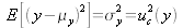 hence, finally:
with
u( x i ) = tandard uncertainty on x i
rij = correlation coefficient of xi and x j
This equation is called propagation of uncertainties law. It shows how the uncertainties u( xi ) of the input quantities xi combine to give the uncertainty uc(y) of the output quantity y.
The partial derivatives
 are called sensitivity coefficients. They describe how the output estimate y en fonction des variations dans les valeurs des estimations d'entrée
x1, x2,...xp
.
are called sensitivity coefficients. They describe how the output estimate y en fonction des variations dans les valeurs des estimations d'entrée
x1, x2,...xp
.
The correlation coefficient rij
is such as
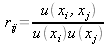 where
where
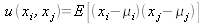 is the covariance of
xi
and
x
.j
is the covariance of
xi
and
x
.j
Non-correlated input quantities
When all the input quantities X1, X2, ...., Xp are independent, that is to say when the covariances u(xi, xj) and the correlation coefficients rij are null, then the combined standard uncertainty is such as:
Cas où Y est une somme ou une différence
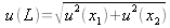
Let distance
L be the quantity depending on the measured quantities position
x
1 et position
x
2 such as
 . Then
 . If
. If
 then
then
 .
.
Case where Y is a product or a quotient
Let illumination
E be the quantity depending on the known or measured quantities intensity
IL and distance
D. Bouguer's law gives
 that is to say :
Correlated input quantities
If the same physical standard scale, the same measuring instrument, the same reference data or the same measuring method is used in the estimate of the input quantities values, then a correlation will exist between input quantities.
In general, if two input quantities X1
and X2
estimated by
x
1
and
x
2
depend on a set of non-correlated variables Q1, Q
2, ..., QL such as
 and,
and,
 , the covariance associated with x1 and x
2 is given by :
, the covariance associated with x1 and x
2 is given by :
with u2(q1) being the variance associated with the estimate q1 of Q1.
The correlation coefficient estimated r(x1,x2) is determined from the expression
with
 and a similar expression for u2(
x2
).
and a similar expression for u2(
x2
).
Ten electric resistors, each of a nominal value Ri=1000Ω re calibrated in comparison with the same standard resistor Rs=1000Ω characterized by a standard uncertainty u(Rs)=100mΩ.
The calibration of each resistor can be represented by the mathematical model
 , with the standard uncertainty
 on the measured ratio
 obtained from replicate observations. We suppose that
 for each resistor and that
 is almost identical for each calibration so that
 .
.
The ten resistors Ri all depend on the same variable Rs because of their calibration. The covariance associated with Ri and Rj is
and
that is to say
Therefore, the correlation coefficient of any two resistors (i≠j) is
The estimated values of the resistors are thus correlated, with a correlation degree which depends on the ratio between the uncertainty of the comparison
 and the uncertainty of the reference standard u(Rs). When the uncertainty of the comparison is negligible in relation to the uncertainty of the standard, the correlation coefficients rij
re equal to +1 and the uncertainty of each calibrated resistor u(Ri) is the same as the one of the standard.
and the uncertainty of the reference standard u(Rs). When the uncertainty of the comparison is negligible in relation to the uncertainty of the standard, the correlation coefficients rij
re equal to +1 and the uncertainty of each calibrated resistor u(Ri) is the same as the one of the standard.
Just as the estimated variance associated with an input quantity includes a statistical component (of Type A) and an evaluated component (of Type B), the estimated covariance associated with two input quantities can also include two contributions of Type A and Type B. Therefore the estimated covariance of two quantities X and Z , which are themselves estimated by the averages
 determined from N independent pairs (x1,zi) of replicate simultaneous observations, is given by
 with
with
The estimated correlation coefficient between the two quantities X andZ ist then
If the frequency of an oscillator with no temperature compensation is an input quantity and if the ambient temperature is also an input quantity and these two quantities are simultaneously observed, then there can be a significant correlation that the calculated covariance of the oscillator's frequency and the ambient temperature will highlight.