Twyman-Green Interferometer
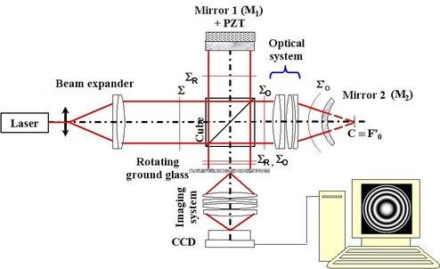
The Twyman Green interferometer is a variant of the Michelson interferometer. It is used industrially for the interferometric control of non-plane optical surfaces and mirrors or lens objectives. Figure 22 presents the Twyman-Green device.
![[zoom...]](javascript:window.open(%22../res/Fig_22_2.jpg%22,%22_blank%22,%22width=%22+Math.min(800,screen.availWidth)+%22,height=%22+Math.min(600,screen.availWidth)+%22,left=%22+(screen.availWidth-800)/2+%22,top=%22+(screen.availHeight-600)/2+%22,scrollbars=yes,resizable=yes%22)?void(0):void(0))
The Michelson plane mirror
 is replaced by a combination of the optical system to study and a spherical mirror. The spherical mirror is placed for its curvature center
 to be confounded with the paraxial focus of the optical system
 . Back and forth in the interferometer, the fringes are visible on the screen that is now replaced by a rotating ground-glass. The optical imagery system creates the fringes image on the
 or
or
 matrix detector. If the ground-glass were static, it would generate a speckle (random phenomenon) that would jam the interference fringes. Thus, the ground-glass is usually assembled on a motor that makes it rotate fast enough for the speckle to be averaged in the integration time of the image sensor so that the speckle grains are no longer visible anymore on the fringes' image.
Reference plane mirror
 is assembled on a piezoelectric transducer which makes it possible to translate
 and to apply the phase shift method in order to calculate the interferences optical phase. This interferometer aspect will not be detailed here but the reader is encouraged to look at the “Interferometry and fringes demodulation” class.
Plane wave surface
 stemming from the laser is split into two plane wave surfaces
 and
and
 . Back and forth on mirror
 , reference wave surface
 remains flat, but it can possibly be sloped by a tilt of mirror
. Object wave surface
remains flat, but it can possibly be sloped by a tilt of mirror
. Object wave surface
 is transformed into a spherical wave by the optical system, if it is perfect, then by reflection on the spherical mirror and back in the optical system, it is flat again. Interferences between the ideal plane wave surface stemming back and forth from mirror
and the wave surface made by the back and forth movement in the optical system occur at the interferometer output. The interference fringes analysis makes it possible to quantify the defect introduced by the optical system.
is transformed into a spherical wave by the optical system, if it is perfect, then by reflection on the spherical mirror and back in the optical system, it is flat again. Interferences between the ideal plane wave surface stemming back and forth from mirror
and the wave surface made by the back and forth movement in the optical system occur at the interferometer output. The interference fringes analysis makes it possible to quantify the defect introduced by the optical system.
Optic component aberration
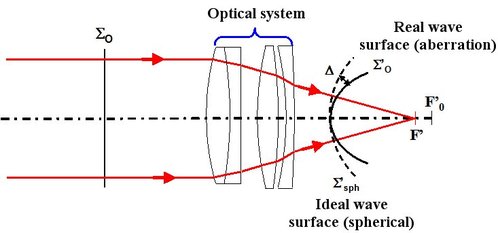
If the optical system tested is perfect then the wave surface stemming from the system-mirror 2 back and forth movement is flat. In the opposite case, it has “aberration” due to the optical system [4.5]. If the optical system is aberrant then the wave surface at the system output is not spherical but has a standard deviation aberration that is the difference between the real wave surface and the ideal spherical wave surface (see figure 23).
![[zoom...]](javascript:window.open(%22../res/Fig_23_1.jpg%22,%22_blank%22,%22width=%22+Math.min(800,screen.availWidth)+%22,height=%22+Math.min(600,screen.availWidth)+%22,left=%22+(screen.availWidth-800)/2+%22,top=%22+(screen.availHeight-600)/2+%22,scrollbars=yes,resizable=yes%22)?void(0):void(0))
The standard deviation aberration depends on the aberration type of the component. A Twyman-Green interferometer easily highlights the following primary aberrations [4.5]:
Third-order spherical aberration
Third-order coma aberration
Third-order astigmatism aberration
The analytic expression of the standard deviation is given in the following examples.
The standard deviation always refers to the difference between the real wave surface and the reference surface that can be either flat or spherical.
Contribution of both mirrors
The reference arm is compounded of plane mirror
assembled on the piezoelectric transducer. A priori, the reflected front that interferes with the measuring wavefront is flat but it may be sloped in relation to the ideal plane. That inclination can be made by a tilting of mirror
.The reader can observe that the same thing occurs with a tilting of mirror
 . If mirror
is slightly translated by the
. If mirror
is slightly translated by the
 then a uniform phase shift of all the reference wavefront points will occur.
 will be the wavefront standard deviation stemming from the reference arm (
 , back and forth).
In the measurement arm, mirror
can be longitudinally tilted or translated. Mirror
longitudinal translation on each side of the optical system paraxial focus will create a defocusing thus a contribution of the mirror to the standard deviation aberration of the optical system-mirror
set will be observed. It is also referred as “focusing defect”.
General expression of the interferogram
Let us suppose that the arms polarizations are parallel so the interferogram is written:
Where :
-
 is the wavefront standard deviation stemming from the measurement arm (optical system+
 , back and forth),
-
is the wavefront standard deviation stemming from the reference arm (
, moving back and forth),
-
 is the optical phase that corresponds to the total difference of optical path between both interferometer paths, assessed at the images sensor level.
According to the contributions given by the various elements, the interferometer fringes will have different shapes.
In the following development, we suppose that
 , that is to say that the fringes have a maximal contrast equal to 1.
Interferogram with a perfect optical system
Let us consider that everything is perfect: optical system, mirror
perpendicular to the optical axis and mirror
perpendicular to the axis and not unfocused. So the contributions standard deviation are
 , the interferogram is:
There is no fringe but “a dull colour”.
As we said it before, the same thing will happen with a tilting of mirror
or
: a wavefront tilt at the output. Let us suppose that the tilting is caused by mirror
. In terms of deviation that wavefront tilt results in the equation a plane so that:
where
 are the mirror tilting angles respectively in directions
 . So the interferogram has straight fringes as illustrated on Figure 12.
Let us consider now that mirror
 is also slightly defocused by a translation
 along the optical axis. The standard deviation caused by that defocusing is written [4.5]:
The notes are illustrated on Figure 24.
![[zoom...]](javascript:window.open(%22../res/Fig_24_1.jpg%22,%22_blank%22,%22width=%22+Math.min(800,screen.availWidth)+%22,height=%22+Math.min(600,screen.availWidth)+%22,left=%22+(screen.availWidth-800)/2+%22,top=%22+(screen.availHeight-600)/2+%22,scrollbars=yes,resizable=yes%22)?void(0):void(0))
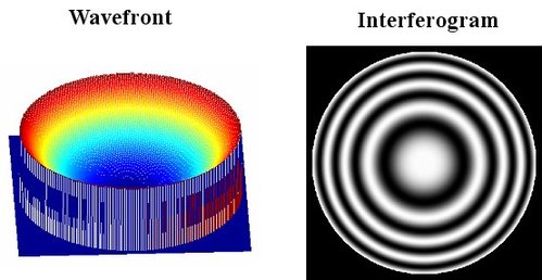
Figure 25 illustrates the wavefront shape and the interferogram obtained with the mirror
defocusing.
![[zoom...]](javascript:window.open(%22../res/Fig_25_1.jpg%22,%22_blank%22,%22width=%22+Math.min(800,screen.availWidth)+%22,height=%22+Math.min(600,screen.availWidth)+%22,left=%22+(screen.availWidth-800)/2+%22,top=%22+(screen.availHeight-600)/2+%22,scrollbars=yes,resizable=yes%22)?void(0):void(0))
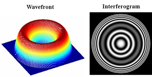
Interferogram with third-order spherical aberration
The spherical aberration is an aperture aberration, that is to say it appears for a image point located on the imager system optical axis whose aperture diameter is wide (numerical aperture wider than 0.35). In the case where the optical system has third-order spherical aberration, the standard deviation is expressed by the following relation [4.5]:
Where
 is the coefficient of the third-order spherical aberration.
Figure 26 illustrates the wavefront shape and the interferogram with third-order spherical aberration.

![[zoom...]](javascript:window.open(%22../res/Fig_26_1.jpg%22,%22_blank%22,%22width=%22+Math.min(800,screen.availWidth)+%22,height=%22+Math.min(600,screen.availWidth)+%22,left=%22+(screen.availWidth-800)/2+%22,top=%22+(screen.availHeight-600)/2+%22,scrollbars=yes,resizable=yes%22)?void(0):void(0))
If mirror
 is now tilted, the wavefronts difference at the interferometer output becomes:
Figure 27 illustrates the wavefront shape and the interferogram with third-order spherical aberration and a tilting of mirror
.
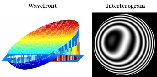
![[zoom...]](javascript:window.open(%22../res/Fig_27_1.jpg%22,%22_blank%22,%22width=%22+Math.min(800,screen.availWidth)+%22,height=%22+Math.min(600,screen.availWidth)+%22,left=%22+(screen.availWidth-800)/2+%22,top=%22+(screen.availHeight-600)/2+%22,scrollbars=yes,resizable=yes%22)?void(0):void(0))
In the case mirror
is slightly defocused, the wavefronts difference at the interferogram output becomes:
Figure 28 illustrates the wavefront shape and the interferogram with third-order spherical aberration and a defocusing of mirror
.
![[zoom...]](javascript:window.open(%22../res/Fig_28_1.jpg%22,%22_blank%22,%22width=%22+Math.min(800,screen.availWidth)+%22,height=%22+Math.min(600,screen.availWidth)+%22,left=%22+(screen.availWidth-800)/2+%22,top=%22+(screen.availHeight-600)/2+%22,scrollbars=yes,resizable=yes%22)?void(0):void(0))
Interferogram with third-order coma aberration
The coma aberration is a field and aperture aberration, that is to say it appears away from the axis. In Figure 22, the configuration it is not possible to highlight the coma. The assembly must be adapted in order to simulate an extended image
 . The optical system must be turned to an angle
 . Thus the parallel to the interferometer axis beams all converge towards image point
 , that can be confounded with mirror
curvature center and the bottom of the image ,
, that can be confounded with mirror
curvature center and the bottom of the image ,
 , as it is located in the system paraxial focus. The image size is
 . The coma standard deviation is expressed by the following relation [4.5]:
Where
 is the third-order coma aberration coefficient.
Figure 29 shows the experimental configuration for the coma measurement.
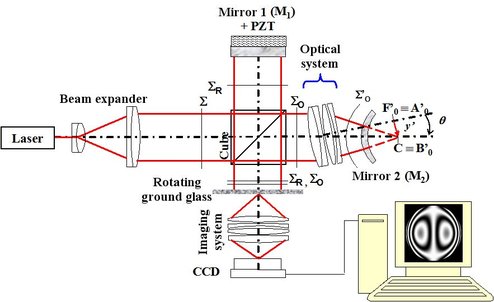
![[zoom...]](javascript:window.open(%22../res/Fig_29_1.jpg%22,%22_blank%22,%22width=%22+Math.min(800,screen.availWidth)+%22,height=%22+Math.min(600,screen.availWidth)+%22,left=%22+(screen.availWidth-800)/2+%22,top=%22+(screen.availHeight-600)/2+%22,scrollbars=yes,resizable=yes%22)?void(0):void(0))
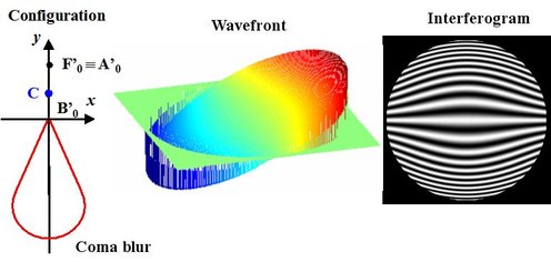
Figure 30 illustrates the wavefront shape and the interferogram with third-order coma aberration. The initial configuration is done in the case where the paraxial image is confounded with the
curvature center: we can also move the curvature center in the coma blur and study the aberration. That move will be done by tilting the mirror
.
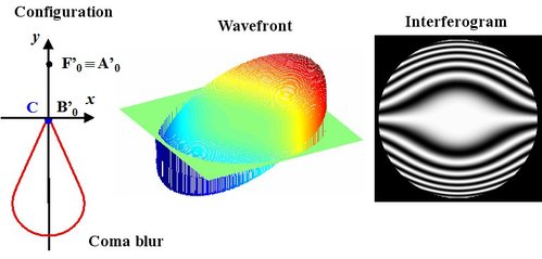
![[zoom...]](javascript:window.open(%22../res/Fig_30_1.jpg%22,%22_blank%22,%22width=%22+Math.min(800,screen.availWidth)+%22,height=%22+Math.min(600,screen.availWidth)+%22,left=%22+(screen.availWidth-800)/2+%22,top=%22+(screen.availHeight-600)/2+%22,scrollbars=yes,resizable=yes%22)?void(0):void(0))
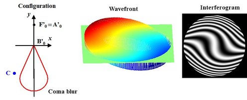
With a tilting of
to put
 out of the coma blur, the aberration wavefront becomes:
Figure 31 illustrates this case.
![[zoom...]](javascript:window.open(%22../res/Fig_31_1.jpg%22,%22_blank%22,%22width=%22+Math.min(800,screen.availWidth)+%22,height=%22+Math.min(600,screen.availWidth)+%22,left=%22+(screen.availWidth-800)/2+%22,top=%22+(screen.availHeight-600)/2+%22,scrollbars=yes,resizable=yes%22)?void(0):void(0))
Figure 32 shows the standard deviation and the interferogram obtained when
is inside the coma blur.

![[zoom...]](javascript:window.open(%22../res/Fig_32_1.jpg%22,%22_blank%22,%22width=%22+Math.min(800,screen.availWidth)+%22,height=%22+Math.min(600,screen.availWidth)+%22,left=%22+(screen.availWidth-800)/2+%22,top=%22+(screen.availHeight-600)/2+%22,scrollbars=yes,resizable=yes%22)?void(0):void(0))
Figure 33 shows the standard deviation and the interferogram obtained when
is moved outside of the meridian plan and outside of the coma blur.
![[zoom...]](javascript:window.open(%22../res/Fig_33_1.jpg%22,%22_blank%22,%22width=%22+Math.min(800,screen.availWidth)+%22,height=%22+Math.min(600,screen.availWidth)+%22,left=%22+(screen.availWidth-800)/2+%22,top=%22+(screen.availHeight-600)/2+%22,scrollbars=yes,resizable=yes%22)?void(0):void(0))
Interferogram with third-order astigmatic aberration
The astigmatic aberration is also a field and aperture aberration that is to say it appears outside the axis for the point. The astigmatic standard deviation is expressed by the following relation [4.5]:
Where
 and
and
 are the tangential and sagittal focus positions in relation to the paraxial focus plan.
Figure 34 illustrates the wavefront shape and the interferogram with third-order astigmatism when the mirror curvature center is confounded with paraxial image
 .
.
![[zoom...]](javascript:window.open(%22../res/Fig_34_1.jpg%22,%22_blank%22,%22width=%22+Math.min(800,screen.availWidth)+%22,height=%22+Math.min(600,screen.availWidth)+%22,left=%22+(screen.availWidth-800)/2+%22,top=%22+(screen.availHeight-600)/2+%22,scrollbars=yes,resizable=yes%22)?void(0):void(0))
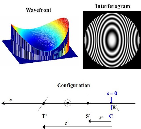
In the case where we defocus spherical mirror
, the standard deviation becomes
For
 , the curvature center is beyond the paraxial image, the wave surface is toric and the fringes are ellipsis as illustrated in Figure 35:

![[zoom...]](javascript:window.open(%22../res/Fig_35_1.jpg%22,%22_blank%22,%22width=%22+Math.min(800,screen.availWidth)+%22,height=%22+Math.min(600,screen.availWidth)+%22,left=%22+(screen.availWidth-800)/2+%22,top=%22+(screen.availHeight-600)/2+%22,scrollbars=yes,resizable=yes%22)?void(0):void(0))
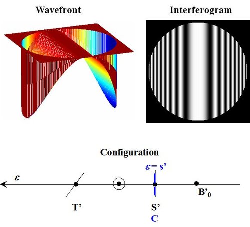
When
 , the wave surface is cylinder-shaped with a vertical axis and the fringes are rectilinear and vertical, mirror
curvature center is on the sagittal focus (Figure 36).
, the wave surface is cylinder-shaped with a vertical axis and the fringes are rectilinear and vertical, mirror
curvature center is on the sagittal focus (Figure 36).
![[zoom...]](javascript:window.open(%22../res/Fig_36_1.jpg%22,%22_blank%22,%22width=%22+Math.min(800,screen.availWidth)+%22,height=%22+Math.min(600,screen.availWidth)+%22,left=%22+(screen.availWidth-800)/2+%22,top=%22+(screen.availHeight-600)/2+%22,scrollbars=yes,resizable=yes%22)?void(0):void(0))
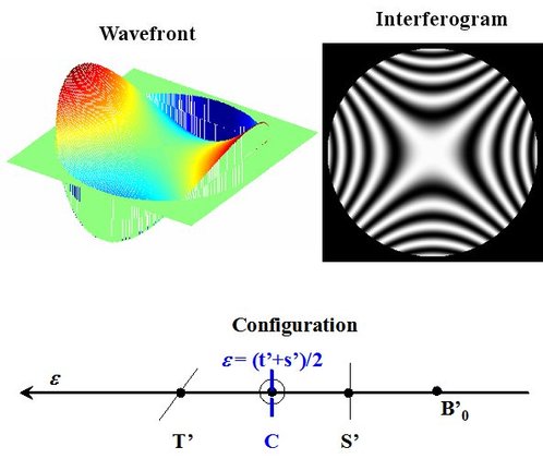
When
 ,the wavefront surface is diabolo-like torus and the fringes are in the shape of crosses, then mirror
curvature center is on the circle with a lesser scattering located half way between sagittal and tangential focuses (Figure 37)
,the wavefront surface is diabolo-like torus and the fringes are in the shape of crosses, then mirror
curvature center is on the circle with a lesser scattering located half way between sagittal and tangential focuses (Figure 37)
![[zoom...]](javascript:window.open(%22../res/Fig_37_1.jpg%22,%22_blank%22,%22width=%22+Math.min(800,screen.availWidth)+%22,height=%22+Math.min(600,screen.availWidth)+%22,left=%22+(screen.availWidth-800)/2+%22,top=%22+(screen.availHeight-600)/2+%22,scrollbars=yes,resizable=yes%22)?void(0):void(0))
When
 ,the wavefront surface is cylinder-like again but with an horizontal axis and the fringes are rectilinear and horizontal, then the mirror
curvature center is on the tangential focus (Figure 38).
,the wavefront surface is cylinder-like again but with an horizontal axis and the fringes are rectilinear and horizontal, then the mirror
curvature center is on the tangential focus (Figure 38).

![[zoom...]](javascript:window.open(%22../res/Fig_38_1.jpg%22,%22_blank%22,%22width=%22+Math.min(800,screen.availWidth)+%22,height=%22+Math.min(600,screen.availWidth)+%22,left=%22+(screen.availWidth-800)/2+%22,top=%22+(screen.availHeight-600)/2+%22,scrollbars=yes,resizable=yes%22)?void(0):void(0))
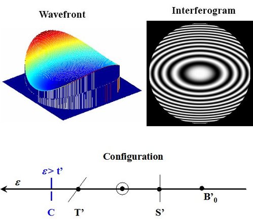
Then, when
 , the mirror curvature center is located between the optical system and the tangential focus, the wave surface is toric again and the fringes are elliptical with a major horizontal axis (figure 39).
![[zoom...]](javascript:window.open(%22../res/Fig_39_1.jpg%22,%22_blank%22,%22width=%22+Math.min(800,screen.availWidth)+%22,height=%22+Math.min(600,screen.availWidth)+%22,left=%22+(screen.availWidth-800)/2+%22,top=%22+(screen.availHeight-600)/2+%22,scrollbars=yes,resizable=yes%22)?void(0):void(0))