Taking the distortions into account
The pinhole camera model modelizes an ideal camera (simple perspective projection) and does not take into account the eventual geometric distortions induced by the optical system used. Several authors [6, 7] proved that it was indispensable to take those distortions into account within applications of dimensional metrology in order to correct them.
The usual parametric approach consists in the modeling of distortion by the improvement of the pinhole camera model with additional terms (thus the model becomes non linear). With this approach, the model draws its inspiration from the geometric aberration theory for a centered (lens) system by adding some corrective terms corresponding to different types of distortions: radial distortion, prismatic distortion, decentering distortion [8, 9, 10].
From the pinhole camera model, the distortions effects can be taken into account by a fourth transformation
 , binding the “ideal” retinal coordinates (2.)
 to the “real“ retinal coordinates
 :
:
Several authors showed that the following model, often called R3D1P1 (3.), is more than enough for most of lens objectives with a focal length superior to 5mm:
where
 is the vector of the distortion parameters.
It is often enough to use a radial model (from order 1 to 3). Writing down:
 , the model R3 is often written as:
We call
 the vector of the intrinsic parameters defined by matrix
 , and
, and
 the vector of the distortion coefficients (which are also intrinsic to the camera):
The model of camera is non-linear and may be written as a vector function
 :
:
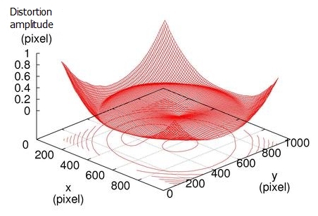
For instance, Figure 5 shows a distortion map (amplitude of the distortion in each pixel of the image) obtained during the calibration of a camera equipped with a 25mm lens objective. This figure perfectly reveals that the main component is the radial distortion (the more we move away from the center of the image, the more the distortion is important). In this example, the distortion is pretty low (the magnitude of the distortion is in the order of 1 pixel at the corners of the image) but it can reach several pixels (or even around 10 pixels) for objectives with lower focal length.
Correction of the distortion
It is sometimes essential to know the ideal pixel coordinates
 , i.e. non-distorted, corresponding to the distorted ones
 .
.
Hence, we can deduce that:
From equations (12) and (13), we notice that it is possible to express
according to
 and the intrinsic parameters
 and
of the camera:
and
of the camera:
In the general case, the distortion model given by equation (14) cannot be inverted and it is therefore necessary to use a numerical method to estimate the ideal coordinates
of the image-point that would have been obtained with a camera exempt from distortion.
Let
 be a pixel of the distorted image. We seek the non distorted pixel
 .
.
The pixel
corresponds to point
 in the retinal plane:
We seek the point
 such as
 :
:
Equation (15) can be resolved thanks to the Newton method applied to the function
 that we initialize with
 .
.
The common iteration is given by the formula:
Namely:
with:
![[zoom...]](javascript:window.open(%22../res/figure_04_1.jpg%22,%22_blank%22,%22width=%22+Math.min(800,screen.availWidth)+%22,height=%22+Math.min(600,screen.availWidth)+%22,left=%22+(screen.availWidth-800)/2+%22,top=%22+(screen.availHeight-600)/2+%22,scrollbars=yes,resizable=yes%22)?void(0):void(0))
![[zoom...]](javascript:window.open(%22../res/figure_05_1.jpg%22,%22_blank%22,%22width=%22+Math.min(800,screen.availWidth)+%22,height=%22+Math.min(600,screen.availWidth)+%22,left=%22+(screen.availWidth-800)/2+%22,top=%22+(screen.availHeight-600)/2+%22,scrollbars=yes,resizable=yes%22)?void(0):void(0))
![[zoom...]](javascript:window.open(%22../res/Eq_C_ext_23_1.jpg%22,%22_blank%22,%22width=%22+Math.min(800,screen.availWidth)+%22,height=%22+Math.min(600,screen.availWidth)+%22,left=%22+(screen.availWidth-800)/2+%22,top=%22+(screen.availHeight-600)/2+%22,scrollbars=yes,resizable=yes%22)?void(0):void(0))
The stop criterion may be based on the value of the error module
 after each iteration. In practice, convergence is reached after only few iterations
 .
.
After obtaining the retinal coordinates
 , the equation (12) is used to enable the calculation of the sought coordinates
 .
.
To calculate a corrected image from a distorted images (which is a different problem from correcting only one point), it is not necessary to use a numerical method in order to invert the distortion model. You just have to use the direct model given by equation (14) and to fill the image-to-draw by sweeping
 and
and
 from the destination image.
For a given pixel
 (in integer coordinates) in the destination image, equation (14) is used to enable the calculation of the coordinates
 of the corresponding point in the source image. Usually, these coordinates are not integer and an interpolation is required in order to calculate the intensity value (grayscale) which must be copied in the destination image at the position
 (cf. [11]).
Other correction methods of distortion have been suggested in the literature. For a review, see in particular the “perspective camera inverse model” section in [12].
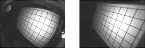
For instance, Figure 6 shows a distorted image (on the left) and the corrected image (on the right).
![[zoom...]](javascript:window.open(%22../res/figure_06_1.jpg%22,%22_blank%22,%22width=%22+Math.min(800,screen.availWidth)+%22,height=%22+Math.min(600,screen.availWidth)+%22,left=%22+(screen.availWidth-800)/2+%22,top=%22+(screen.availHeight-600)/2+%22,scrollbars=yes,resizable=yes%22)?void(0):void(0))
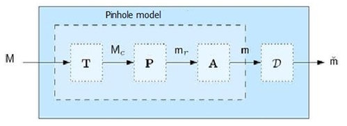
Non-parametric approach
In the case of complex optical systems, some authors [13] have proved that it is recommended to modelize the distortion in a non-parametric way using spline functions [14].
In that case, it is a purely mathematical modeling (kind of “black box” approach) aiming to determine the distortion function that shows the best the way in which the ideal image is distorted [15, 16].
As it is a purely mathematical modeling (4.), it is not a problem to adopt the layout of Figure 7 and to seek the distortion function
 that links the ideal image-coordinates
 of point
 to the image-coordinates
 of point
 .
.
![[zoom...]](javascript:window.open(%22../res/figure_07_1.jpg%22,%22_blank%22,%22width=%22+Math.min(800,screen.availWidth)+%22,height=%22+Math.min(600,screen.availWidth)+%22,left=%22+(screen.availWidth-800)/2+%22,top=%22+(screen.availHeight-600)/2+%22,scrollbars=yes,resizable=yes%22)?void(0):void(0))
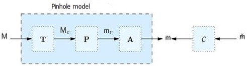
In this approach, to be able to correct the distortion easily, it is better to choose the model schematically presented on Figure 8, in which the reciprocal function
 of distortion correction is used instead of the distortion function
 . Indeed, the distortion can be corrected directly using
hereas it may require a lot of time to do all the calculations in the case of inverting function
, particularly when its reciprocal function
cannot be analytically determined. Moreover, the field of definition of the spline function for the correction of
is a priori known and determined by the dimension of the images, whereas the spline function for the distortion of
has an a priori unknown definition field since it is expressed in the retinal plane which is defined by the calibration.
. Indeed, the distortion can be corrected directly using
hereas it may require a lot of time to do all the calculations in the case of inverting function
, particularly when its reciprocal function
cannot be analytically determined. Moreover, the field of definition of the spline function for the correction of
is a priori known and determined by the dimension of the images, whereas the spline function for the distortion of
has an a priori unknown definition field since it is expressed in the retinal plane which is defined by the calibration.
![[zoom...]](javascript:window.open(%22../res/figure_08_1.jpg%22,%22_blank%22,%22width=%22+Math.min(800,screen.availWidth)+%22,height=%22+Math.min(600,screen.availWidth)+%22,left=%22+(screen.availWidth-800)/2+%22,top=%22+(screen.availHeight-600)/2+%22,scrollbars=yes,resizable=yes%22)?void(0):void(0))
The equation of the distortion correction becomes:
The estimation of the function of distortion correction
consists in approximating horizontal (following the axis
 ) and vertical (following the axis
 ) components of the distortion correction field by two spline surfaces
 and
[13, 17].
and
[13, 17].
The function of distortion correction permits to correct the points (or a full image) from their distortion. The corrected points are linked to the 3D entry points by a classical pinhole model the parameters of which are easy to estimate.
We are done with establishing the linear (5) and non-linear (11) models of a camera, we are now going to deal with the calibration methods that permit to estimate the parameters of these models.